OpenSim Models

The topics covered in this section include:

Overview

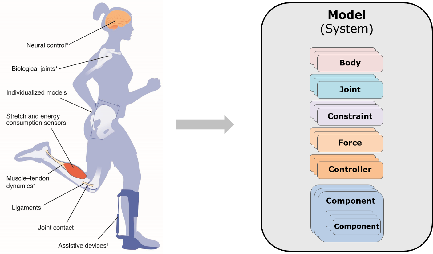
An OpenSim model represents the neuromuscular and musculoskeletal dynamics of a human or animal that is of interest to study within a computer simulation. The OpenSim model is made up of components corresponding to parts of the physical system that combine to generate or describe movement. These parts are: reference frames, bodies, joints, constraints, forces, contact geometry, markers and controllers. 

In OpenSim, a model's skeletal system is represented by rigid bodies interconnected by joints. Joints define how two bodies (e.g., bone segment), termed parent and child bodies, can move with respect to one another. Constraints can also be applied to limit the motion of bodies. 

Muscles are modeled as specialized force elements that act at muscle points (e.g., insertion and origin points) connected to rigid bodies. The force of a muscle is typically dependent on the path through muscle points comprised of muscle fiber and tendon lengths, the rate of change of the fiber lengths, and the level of muscle activation. OpenSim also has a variety of other forces, which represent externally applied forces (e.g., ground reaction forces), passive spring-dampers (e.g., ligaments), and controlled linear and torsional actuators.

The figure below shows a conceptual schematic of an OpenSim model. In the remainder of the chapter, we will discuss the OpenSim model file format used to describe these models.You can edit these properties using scripts (in the GUI, Matlab or Python), via an XML editor, or you can view and edit the properties using the GUI Property Editor and Outputs List.

OpenSim Model File Format

An OpenSim model is described by a file that utilizes the XML code structure to organize its contents. XML uses tags to identify and manage information, such as:

<gravity>0 -9.8065999999999995 0</gravity>

where <gravity> signifies the opening of the tag, 0 -9.8065999999999995 0 is a vector describing the acceleration due to gravity, and </gravity> signifies the end of the tag. The name of the tag identifies the type of information between the tags. When you edit an OpenSim model file, there are tags representing each part of the model, as shown in the figure below. 

An OpenSim Model File (arm26.osim).  The file below was opened in the XML editor Notepad++, which provides the color syntax highlighting.  The sections have been collapsed to highlight the model components.  Clicking on the + icon to the left of a section would expand it, displaying the relevant tags for that section.

Connecting Components Together using Sockets and Component Paths

It is common for components to depend on each other. For example, Joint components depend on the Body components (actually, PhysicalFrames) that the Joint connects. To specify these dependencies, OpenSim uses the notion of Sockets. As you will see later, a Joint has two Sockets: parent_frame and child_frame. You can specify the frames that satisfy these sockets in XML:

<socket_parent_frame>/ground</socket_parent_frame>
<socket_child_frame>/bodyset/r_humerus</socket_child_frame>

Any XML element whose tag begins with socket_ is used to indicate the path to a component (ComponentPath) in the model that should be used to satisfy the socket. Models in OpenSim version 4.0 and greater are hierarchical: components can contain other components. For example, the BodySet component named 'bodyset' contains the Body component 'r_humerus'. We use forward slashes, similar to a file system path or web URL, to indicate the path to a component in the model's hierarchy. In the example above, we use absolute paths (starting with a slash), but relative paths (e.g., ../../some/other/component) also work.

Bodies

In formulating the equations-of-motion (i.e., the system dynamics), OpenSim employs Simbody which is an open-source multibody dynamics solver. In Simbody and OpenSim, the body is the primary building block of the model. Each body in turn owns a joint that connects it to an existing parent body. The joint defines the coordinates and kinematic transforms that govern the motion of that body with respect to its parent body. Within the model all bodies are contained in a BodySet. 

Thus, to start our model, we need to define a set of rigid bodies that represent our system. In the <BodySet> section, we define this group of bodies, with the name, mass properties, and visible objects associated with each body. The figure below shows an example of the r_humerus body in the Arm26 model. Note the key tags, such as <mass>, <mass_center>, and <inertia> (and similarly named tags for inertia in other directions).

Example XML Code from Model Arm26 to Represent a Body

<Body name="r_humerus">
	<attached_geometry>...</attached_geometry>
	<WrapObjectSet>...</WrapObjectSet>
	<mass>1.8645719999999999</mass>
	<mass_center>0 -0.18049599999999999 0</mass_center>
	<inertia>0.01481 0.0045510000000000004 0.013193 0 0 0</inertia>
</Body>

Every model comes with a Ground body, which exists as a property of a Model, not in the BodySet.

Geometry

<Body>
  <.....>
  <!--List of geometry attached to this Frame. Note, the 
    geometry are treated as fixed to the frame and they share the transform of 
    the frame when visualized-->
  <attached_geometry>
		<!-- Mesh geometry comes from a file -->
    	<Mesh name="base_geom_1">
		<!--Path to a Component that satisfies the Socket 'frame' of type Frame.-->
		<socket_frame>..</socket_frame>
		<!--Path to an output (channel) to satisfy the one-value Input 'transform' of type SimTK::Transform (description: The transform that positions the Geometry in Ground so it can be positioned. Note, either the Geometry is attached to a Frame OR the input transform can be supplied, but not both. ).-->
		<input_transform></input_transform>
		<!--Scale factors in X, Y, Z directions respectively.-->
		<scale_factors>1 1 1</scale_factors>
		<!--Default appearance attributes for this Geometry-->
		<Appearance>
			<!--Flag indicating whether the associated Geometry is visible or hidden.-->
			<visible>true</visible>
			<!--The opacity used to display the geometry between 0:transparent, 1:opaque.-->
			<opacity>1</opacity>
			<!--The color, (red, green, blue), [0, 1], used to display the geometry. -->
			<color>1 1 1</color>
			<!--Visuals applied to surfaces associated with this Appearance.-->
			<SurfaceProperties>
				<!--The representation (1:Points, 2:Wire, 3:Shaded) used to display the object.-->
				<representation>3</representation>
			</SurfaceProperties>
		</Appearance>
		<!--Name of geometry file.-->
		<mesh_file>bone.vtp</mesh_file>
	</Mesh>
	<Sphere>
		<radius>1.5</radius>
	<Sphere>
    <...>
  </attached_geometry>
  <....>
</Body>

Joints

In addition to the set of rigid bodies, we also need to define the relationship between those bodies (i.e., joint definitions). In the figure below, a joint (in red) defines the kinematic relationship between two frames (B and P) each affixed to a rigid-body (the parent, P_o, and the body being added, B_o) parameterized by joint coordinates 

A body is a moving reference frame (B_o) in which its center-of-mass and inertia are defined, and the location of a joint frame (B) fixed to the body can be specified. Similarly, the joint frame (P) in the parent body frame (P_o) can also be specified. Flexibility in specifying the joint is achieved by permitting joint frames that are not coincident with the body frame. In 4.0, this flexibility was enhanced via the introduction of the Frame class hierarchy. There are three main types of Frames: Ground (each model starts with a ground frame), Body, and PhysicalOffsetFrame. All three of these frames are called PhysicalFrames because they either are a rigid body or are fixed to a rigid body. In OpenSim 4.0, a joint connects two PhysicalFrames (parent and child). One can use PhysicalOffsetFrames to specify a constant transform between a joint frame and the body frame.

The figure below shows an example from Arm26 defining the r_shoulder joint. Note the key tags, such as <socket_parent_frame>, <socket_child_frame>, <Coordinate>, <translation>, and <orientation>. Note the use of an intermediate PhysicalOffsetFrame for the joint's parent frame.

<CustomJoint name="r_shoulder">
	<socket_parent_frame>base_offset</socket_parent_frame>
	<socket_child_frame>/bodyset/r_humerus</socket_child_frame>
	<coordinates>
		<Coordinate name="r_shoulder_elev">
			<default_value>0</default_value>
			<default_speed_value>0</default_speed_value>
			<range>-1.5707963300000001 3.1415926500000002</range>
			<clamped>false</clamped>
			<locked>false</locked>
			<prescribed_function />
		</Coordinate>
	</coordinates>
	<frames>
		<PhysicalOffsetFrame name="base_offset">
			<socket_parent>/bodyset/base</socket_parent>
			<translation>-0.017545000000000002 -0.0070000000000000001 0.17000000000000001</translation>
			<orientation>0 0 0</orientation>
		</PhysicalOffsetFrame>
	</frames>
	<SpatialTransform>...</SpatialTransform>
</CustomJoint>

Available Joint Types

1. WeldJoint: introduces no coordinates (degrees of freedom) and fuses bodies together
2. PinJoint: one coordinate about the common Z-axis of parent and child joint frames
3. SliderJoint: one coordinate along common X-axis of parent and child joint frames
4. BallJoint: three rotational coordinates that are about X, Y, Z of B in P
5. EllipsoidJoint: three rotational coordinates that are about X, Y, Z of B in P with coupled translations such that B traces and ellipsoid centered at P
6. FreeJoint: six coordinates with 3 rotational (like the ball) and 3 translations of B in P
7. CustomJoint: user specified 1-6 coordinates and user defined spatial transform to locate B with respect to P

The CustomJoint Transform

Most joints in an OpenSim model are custom joints since this is the most generic joint representation, which can be used to model both conventional (pins, slider, universal, etc.) as well as more complex biomechanical joints. The user must define the transform (rotation and translation) of the child in the parent (B and P, in the joint definition figure above) as a function of the generalized coordinates listed in the Joint’s CoordinateSet. Consider the spatial transform  :

where

q are the joint coordinates, and x are the spatial coordinates for the rotations (x₁, x₂, x₃) and translations (x₄, x₅, x₆) along user-defined axes that specify a spatial transform (X) according to functions f_i. The behavior of a CustomJoint is specified by its SpatialTransform. A SpatialTransform is comprised of 6 TransformAxis tags (3 rotations and 3 translations) that define the spatial position of B in P as a function of coordinates. Each transform axis enables a function of joint coordinates to operate about or along its axis. The function of q is used to determine the displacement for that axis. The order of the spatial transform is fixed with rotations first followed by translations. Subsequently, coupled motion (i.e., describing motion of two degrees of freedom as a function of one coordinate) is easily handled. The example below (from the gait2354.osim model) describes coupled motion of the knee, with both tibial translation and knee flexion described as a function of knee angle: 

<SpatialTransform name="">
  <!--3 Axes for rotations are listed first.-->
  <TransformAxis name="rotation1">
    <function>
      <LinearFunction name="">
        <coefficients> 1.00000000 0.0000000 </coefficients>
      </LinearFunction>
    </function> 
    <coordinates> knee_angle_r </coordinates>
    <axis> 0.00000000 0.00000000 1.00000000 </axis>
  <TransformAxis>
 
  <TransformAxis name="rotation2">
    <function>
      <Constant name="">
        <value> 0.00000000 </value> 
      </Constant>
    </function>
    <coordinates> </coordinates>
    <axis> 0.00000000 1.00000000 0.00000000 </axis>
  </TransformAxis>
 
  <TransformAxis name="rotation3"> ...
 
  <!--3 Axes for translations are listed next.-->
  <TransformAxis name="translation1">
    <function>
      <NaturalCubicSpline name=""> ...
    </function>
    <coordinates> knee_angle_r </coordinates>
    <axis> 1.00000000 0.00000000 0.00000000 </axis>
   </TransformAxis>
 
  <TransformAxis name="translation2">
    <function>
      <NaturalCubicSpline name=""> ... 
    </function>
    <coordinates> knee_angle_r </coordinates>
    <axis> 0.00000000 1.00000000 0.00000000 </axis>
  </TransformAxis>
 
  <TransformAxis name="translation3"> ...
</SpatialTransform>

Kinematic Constraints in OpenSim

OpenSim currently supports three types of built-in constraints: PointConstraint, WeldConstraint, and CoordinateCouplerConstraint. A point constraint fixes a point defined with respect to two bodies (i.e., no relative translations). A weld constraint fixes the relative location and orientation of two bodies (i.e., no translations or rotations). A coordinate coupler relates the generalized coordinate of a given joint (the dependent coordinate) to any other coordinates in the model (independent coordinates). The user must supply a function that returns a dependent value based on independent values. The following example implements coordinate coupler constraint for the motion of the patella as a function of the knee angle and also welds the foot to ground.

<!--Constraints in the model.-->
<ConstraintSet name="">
	<objects>
		<!-- Constrain the translation of the patella in the x-direction as a function of the knee_angle -->
		<CoordinateCouplerConstraint name="pat_tx_r">
			<isEnforced> true </isEnforced>
				<coupled_coordinates_function>
					<SimmSpline name="">
						<x>  -2.09439510  -1.39626340  -1.04719755  -0.69813170  -0.34906585  -0.17453293  ...  </x>
						<y>   0.01710145   0.03202815   0.03766273   0.04250649   0.04636173   0.04784451  ...  </y>
					</SimmSpline>
                </coupled_coordinates_function>
				<!-- coordinates involved in the constraint must be defined by joints in this model -->
                <independent_coordinate_names> knee_angle_r </independent_coordinate_names>
                <dependent_coordinate_name> pat_tx_r </dependent_coordinate_name>
		</CoordinateCouplerConstraint>

		<!-- Constrain the translation of the patella in the y-direction as a function of the knee_angle -->
        <CoordinateCouplerConstraint name="pat_ty_r"> ...
		
		<!-- Constrain the rotation of the patella as a function of the knee_angle -->        
		<CoordinateCouplerConstraint name="pat_angle_r"> ...
  
		<!-- Constrain a foot to the floor with a weld. A weld specifies a location and orientation of two frames
			 on separate bodies that must remain spatially coincident and aligned. --> 
    	<WeldConstraint name="weld">
			<isEnforced>true</isEnforced>
			<socket_frame1> /bodyset/foot_r </socket_frame1>
			<socket_frame2> /ground </socket_frame2>
		</WeldConstraint>
	</objects>
	<groups/>
</ConstraintSet>

Forces

In order to actuate our model, we need to define the forces that will be applied to the model. Just like bodies are defined within the <BodySet> section, forces are defined in the <ForceSet> section of the model file. Forces come in two varieties: passive forces like springs, dampers, and contact and active forces like springs, idealized linear or torque actuators, and muscles. Active forces that require input (controls) supplied by the user or by a controller are called Actuators and are a subset of the ForceSet. 

Available Forces

OpenSim has several built-in forces that include: PrescribedForce, SpringGeneralizedForce, BushingForce, as well as HuntCrossleyForce and ElasticFoundationForce to model forces due to contact (Note: contact forces also require defining contact geometry). Below is an example of a bushing force used to model passive structures surrounding a single lumbar joint that connects a torso body to a pelvis body.

<BushingForce>
	<appliesForce>true</appliesForce>
	<socket_frame1></socket_frame1>
	<socket_frame2></socket_frame2>
	<rotational_stiffness>0 0 0</rotational_stiffness>
	<translational_stiffness>0 0 0</translational_stiffness>
	<rotational_damping>0 0 0</rotational_damping>
	<translational_damping>0 0 0</translational_damping>
</BushingForce>

Common Actuators

OpenSim also includes “ideal” actuators which apply pure forces or torques that are directly proportional to the input control (i.e., excitation) via its optimal force (i.e., a gain). Forces and torques are applied between bodies, while generalized forces are applied along the axis of a generalized coordinate (i.e., a joint axis).

<!--Apply a force at a point in the direction specified in the body frame -->
<PointActuator name="FY_residual">
 <!--Name of Body to which this actuator is applied.-->
 <body> pelvis </body>
 <!--Location of application point; in body frame unless point_is_global=true-->
 <point> 0 0 0</point>
 <!--Interpret point in Ground frame if true; otherwise, body frame.-->
 <point_is_global> false </point_is_global>
 <!--Force application direction; in body frame unless force_is_global=true.-->
 <direction> 1 0 0</direction>
 <!--Interpret direction in Ground frame if true; otherwise, body frame.-->
 <force_is_global> true </force_is_global>
 <!--The maximum force produced by this actuator when fully activated.-->
 <optimal_force> 8.0 </optimal_force>
</PointActuator>
  
 <!--Apply an equal and opposite torque on two bodies about the axis defined in the the first body -->
<TorqueActuator name="MZ_residual">
 <optimal_force> 1000.0 </optimal_force>
 <bodyA> ground </bodyA>
 <axis> 0.000 0.000 -1.000 </axis>
 <bodyB> pelvis </bodyB>
</TorqueActuator >
 
<!--Apply a generalized force along (force) or about (torque) the axis of a generalized coordinate. Positive force increases the coordinate -->
<CoordinateActuator name="knee_reserve">
 <optimal_force> 300.0 </optimal_force>
 <coordinate> knee_angle_r </coordinate>
</CoordinateActuator>

The Muscle Actuator

There are several muscle models in OpenSim. All muscles include a set of muscle points where the muscle is connected to bones (bodies) and provide utilities for calculating muscle-actuator lengths and velocities. Internally muscle models may differ in the number and types of parameters. Muscles typically include muscle activation and contraction dynamics and their own states (for example activation and muscle fiber length). The control values are typically bounded excitations (ranging from 0 to 1) which lead to a change in activation and then force. Below is an example of a muscle model, as described by Thelen (2003), from an OpenSim model. 

In addition to the muscle properties, we need to define its geometry. In this example, a geometry path is defined for the muscle using a set of path points.

<Thelen2003Muscle name="BICshort">
	<appliesForce>true</appliesForce>
	<!--The set of points defining the path of the actuator.-->
	<GeometryPath>
		<!--The set of points defining the path-->
		<PathPointSet>
			<objects>
				<PathPoint name="BICshort-P1">
					<socket_parent_frame>/bodyset/base</socket_parent_frame>
					<!--The fixed location of the path point expressed in its parent frame.-->
					<location>0.0046750000000000003 -0.01231 0.13475000000000001</location>
				</PathPoint>
				<PathPoint name="BICshort-P2">
					<socket_parent_frame>/bodyset/base</socket_parent_frame>
					<!--The fixed location of the path point expressed in its parent frame.-->
					<location>-0.0070749999999999997 -0.040039999999999999 0.14507</location>
				</PathPoint>
				...
		</PathPointSet>
		<!--The wrap objects that are associated with this path-->
		<PathWrapSet>...</PathWrapSet>
		<!--Default appearance attributes for this GeometryPath-->
		<Appearance>
			<!--The color, (red, green, blue), [0, 1], used to display the geometry. -->
			<color>0.80000000000000004 0.10000000000000001 0.10000000000000001</color>
		</Appearance>
	</GeometryPath>
	<!--Maximum isometric force that the fibers can generate-->
	<max_isometric_force>435.56</max_isometric_force>
	<!--Optimal length of the muscle fibers-->
	<optimal_fiber_length>0.1321</optimal_fiber_length>
	<!--Resting length of the tendon-->
	<tendon_slack_length>0.1923</tendon_slack_length>
	<!--Angle between tendon and fibers at optimal fiber length expressed in radians-->
	<pennation_angle_at_optimal>0</pennation_angle_at_optimal>
	<!--Maximum contraction velocity of the fibers, in optimal fiberlengths/second-->
	<max_contraction_velocity>10</max_contraction_velocity>
	<!--tendon strain at maximum isometric muscle force-->
	<FmaxTendonStrain>0.033000000000000002</FmaxTendonStrain>
	<!--passive muscle strain at maximum isometric muscle force-->
	<FmaxMuscleStrain>0.59999999999999998</FmaxMuscleStrain>
	<!--shape factor for Gaussian active muscle force-length relationship-->
	<KshapeActive>0.5</KshapeActive>
	<!--exponential shape factor for passive force-length relationship-->
	<KshapePassive>4</KshapePassive>
	<!--force-velocity shape factor-->
	<Af>0.29999999999999999</Af>
	<!--maximum normalized lengthening force-->
	<Flen>1.8</Flen>
	<!--Activation time constant, in seconds-->
	<activation_time_constant>0.01</activation_time_constant>
	<!--Deactivation time constant, in seconds-->
	<deactivation_time_constant>0.040000000000000001</deactivation_time_constant>
</Thelen2003Muscle>

Markers

In order to perform Inverse Kinematics, you will need to define a virtual marker set that matches the experimental marker set used to collect motion capture data. Markers are defined in a <MarkerSet>. The figure below (Example XML Marker) shows an example from Arm26 defining a <Marker>. Note tags that define the marker, such as <socket_parent_frame> and <location>. Additionally, the marker name is important, as it must match the name of the corresponding experimental marker.

<Marker name="r_acromion">
	<socket_parent_frame>/bodyset/base</socket_parent_frame>
	<location>-0.01256 0.040000000000000001 0.17000000000000001</location>
	<fixed>false</fixed>
</Marker>

Contact Geometry

A model may have some specific contact geometry that is associated with a model. In OpenSim, contact geometry can be an analytical shape, such as a half-place, sphere, or cube, or a user-defined shape represented in a geometry file. Files of type .obj, .stl, and .vtp are supported as of version 3.3. Prior versions of OpenSim support only .obj files. The figure below shows an example defining contact for the ground (half-space) and a user-defined block from the tugOfWar model. Note tags that define the contact object, such as <socket_frame>, <location>, <orientation>, and <filename>.

Example XML Code from Model tugOfWar to Represent Contact Geometry

<ContactGeometrySet>
	<objects>
		<ContactHalfSpace>
			 <socket_frame>/ground</socket_frame>
			 <location>0 0 0</location>
			 <orientation>0 0 0</orientation>
			 <Appearance>
				 <visible>true</visible>
				 <opacity>1</opacity>
				 <color>0 1 1</color>
				 <SurfaceProperties>
					 <representation>2</representation>
				 </SurfaceProperties>
			 </Appearance>
		 </ContactHalfSpace>
		 <ContactMesh>
			  <socket_frame>/bodyset/block</socket_frame>
			  <location>0 0 0</location>
			  <orientation>0 0 0</orientation>
			  <Appearance>
				  <visible>true</visible>
				  <opacity>1</opacity>
				  <color>0 1 1</color>
				  <SurfaceProperties>
					  <representation>2</representation>
				  </SurfaceProperties>
			  </Appearance>
			  <filename>blockRemesh192.obj</filename>
		  </ContactMesh>
	</objects>
	<groups />
</ContactGeometrySet>