Tutorial 3 - Scaling, Inverse Kinematics, and Inverse Dynamics

The tutorial below is designed for use with OpenSim version 4.0 and later. A version of the tutorial compatible with OpenSim version 3.3 is available here.

I. Objectives

Purpose

The purpose of this tutorial is to demonstrate how OpenSim solves an inverse kinematics and dynamics problem using experimental data. To diagnose movement disorders and study human movement, biomechanists frequently ask human subjects to perform movements in a motion capture laboratory and use computational tools to analyze these movements. A common step in analyzing a movement is to compute the joint angles and joint moments of the subject during movement. OpenSim has tools for computing these quantities:

Inverse kinematics is used to compute joint angles.
Inverse dynamics is used to compute net joint reaction forces and net joint moments.

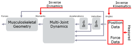
Inverse kinematics computes the joint angles for a musculoskeletal model that best reproduce the motion of a subject. Inverse dynamics then uses joint angles, angular velocities, and angular accelerations of the model, together with the experimental ground reaction forces and moments, to solve for the net reaction forces and net moments at each of the joints. The schematic below shows an overview of the inverse kinematics and inverse dynamics problems.

In this tutorial, you will:

Become familiar with OpenSim's Scale, Inverse Kinematics and Inverse Dynamics tools
Solve an inverse kinematics and inverse dynamics problem using experimental data
Interpret the results of the inverse dynamics solution
Investigate the dynamic inconsistencies that arise during inverse dynamics

Format

Each section of the tutorial guides you in using certain tools within and asks you to answer a few questions. The menu titles and option names you must select and any commands you must type to run OpenSim will appear in bold face. The questions can be answered based on information from OpenSim and basic knowledge of the human musculoskeletal system. After you complete the tutorial, feel free to explore OpenSim and the other analysis tools further on your own. Depending on the amount of exploration you do, this tutorial should take 1-2 hours to complete.

II. Generic Musculoskeletal Model

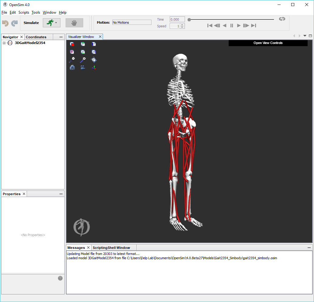
In this tutorial, you will be using a generic musculoskeletal model with 23 degrees of freedom and actuated by 54 muscles entitled 3DGaitModel2354.
Note: Detailed information about the model can found on the Gait2392 and 2354 Models page

To load the generic musculoskeletal model into OpenSim:

Click the File menu and select Open Model.

Find the Gait2354_Simbody folder in your default OpenSim resources directory— \Documents\OpenSim\Models for PC and Mac.
Note: When you first launch OpenSim, you are prompted to provide a path to install the resources folder, the default is in your systems Documents folders.

Open the Gait2354_Simbody folder, select the file gait2354_simbody.osim, and click Open.

III. Scaling A Musculoskeletal Model

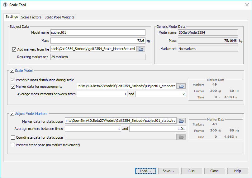
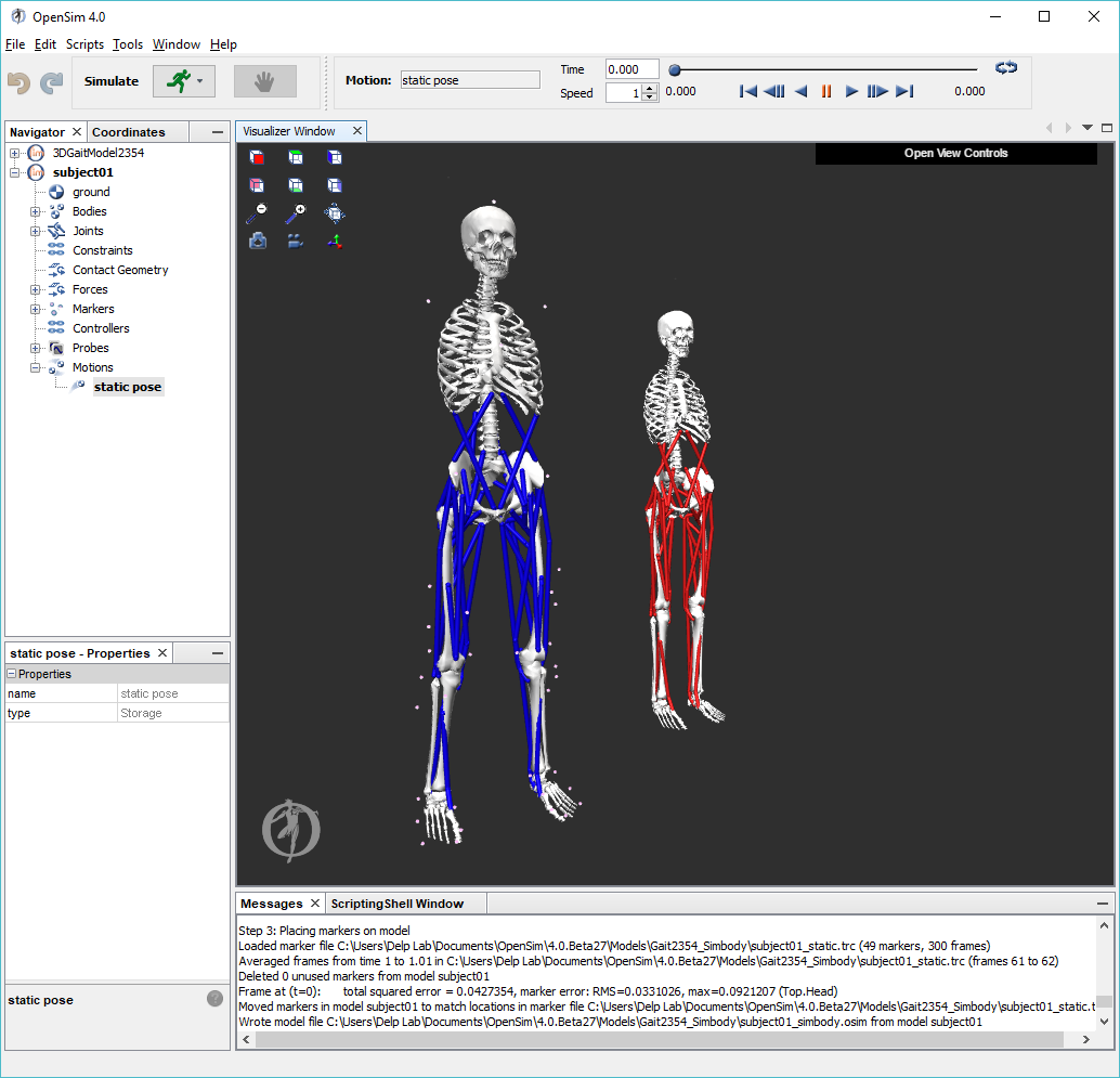
Subject specific modeling involves (i) scaling a generic musculoskeletal model to modify the anthropometry, or physical dimensions, of the generic model so that it matches the anthropometry of a particular subject and (ii) registering the markers placed on the model to match the locations on the subject. Scaling and Registration are the most important steps in solving inverse kinematics and inverse dynamics problems because IK and ID solutions are sensitive to the accuracy of the scaling and registration.

To scale the generic model and register the markers:

Click the Tools menu and select Scale Model.
At the bottom of the Scale Tool dialog, click Load to input a settings file.
In the file browser, ensure that you are in the Gait2354 folder, select the file subject01_Setup_Scale.xml and click Open.

This Scale Setup file is an xml file that contains pre-configured settings to scale and register the generic gait2354 musculoskeletal model to the dimensions of a subject that we have experimental data for. A detailed explanation of the Scale Tool can be found on the Scaling page of the documentation.

Model Scaling

In OpenSim, the scaling step adjusts both the dimensions of the body segments, as well as the mass properties (mass and inertia tensor). Scaling can be performed using a combination of two methods:

(1) Manual Scaling: Scaling that allows the user to scale a segment based on some predetermined scale factor. Manual scaling is sometimes necessary when suitable data are not available, or if the scale factors were determined using an alternative algorithm.

(2) Measurement-based Scaling: Scaling that determines scale factors for a body segment by comparing distance measurements between specified landmarks on the model, known as model markers, and the corresponding experimental marker positions.

Marker Registration

In, OpenSim, the registration step adjusts the location of model markers to match the location of markers on the subject. To do this, you must first estimate a pose for the model that closely resembles the pose of the subject during the experimental static trial.

To complete the scale step:

In the Scale Tool dialog, click Run.
When complete, a new, scaled and registered model entitled subject01 will appear in Visualizer window. Notice the pink model markers around the new model.

To save the scaled model, either click File and select Save Model, or right-click on the model name, subject01, in the Navigator window, and select Save As.

Save the scaled model as gait2354_scaled.osim, and click Save.
Note: ensure that you are in the Gait2354 folder.
Once you have answered Questions 1-5, below, close the Scale Tool Dialog by clicking Close. At this point, you may close the generic model (right-click the model name in the Navigator window, and select Close) or hide the model (right-click the model name, and select Display -> Hide).

Questions

1. Based on information in the Scale Tool dialog, what is the mass of the generic musculoskeletal model? What was the mass of the subject?

2. What frequency was the experimental motion data captured?
Hint: Look for the box titled Marker Data.

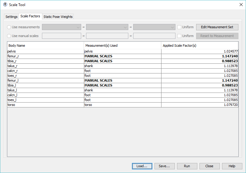
3. Click on the Scale Factors tab. Which body segments were scaled manually?

4. In the Scale Factors Tab, click on the Edit Measurements Set. Which marker pairs are used to determine the Right Femur scaling? Is this a good assumption? When is this not a good assumption?

5. Click on the Static Pose Weights tab. Which markers are used to determine the pose of the model?

IV. Inverse Kinematics

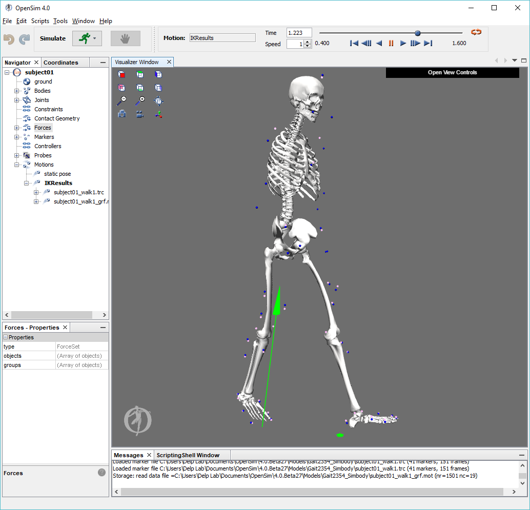
Kinematics is the study of motion without considering the forces and moments that produce that motion. The purpose of inverse kinematics (IK) is to estimate the joint angles of a particular subject from experimental data. In this section, you will estimate a subject's joint angles during walking by performing an IK analysis using the subject scaled model and experimentally collected walking data.

For each time step of recorded motion data, IK computes a set of joint angles that put the model in a configuration that "best matches" the experimental kinematics. OpenSim determines this "best match" by solving a weighted least squares optimization problem with the goal of minimizing marker error. Marker error is defined as the distance between an experimental marker and the corresponding model marker. Each marker has an associated weighting value, specifying how strongly that marker's error term should be minimized in the least squares problem. For each time step, the inverse kinematics tool solves for a vector of generalized coordinates (e.g., joint angles), q, that minimizes the weighted sum of marker errors, which is expressed as

where q is the vector of generalized coordinates (e.g., joint angles), x_i^exp is the position of experimental marker i, x_i(q) is the position of the corresponding model marker i (which depends on q), and w_i is the weight associated with marker i.

To setup an inverse kinematics analysis:

Open the Inverse Kinematics Tool dialog window by clicking the Tools menu and selecting Inverse Kinematics.

Load an inverse kinematics tool setup file by clicking Load, selecting the file subject01_Setup_IK.xml, and clicking Open.
Note: In the file browser, ensure that you are in the Gait2354_Simbody folder,

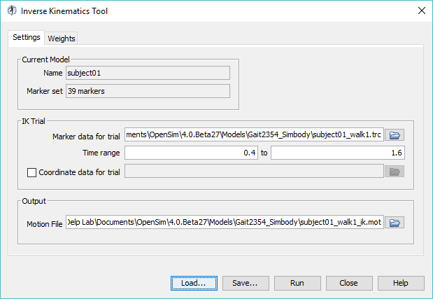
subject01_Setup_IK.xml contains pre-configured settings for the inverse kinematics tool. Notice the text boxes in the dialog window are now are filled with values. A detailed explanation of the Inverse Kinematics Tool can be found on the Inverse Kinematics page of the documentation.

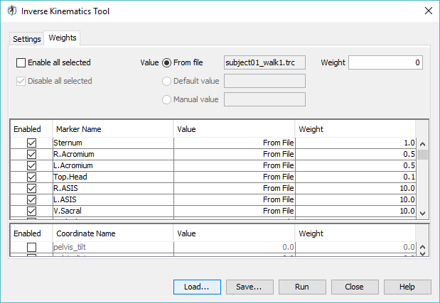
Navigate to the Weights tab.

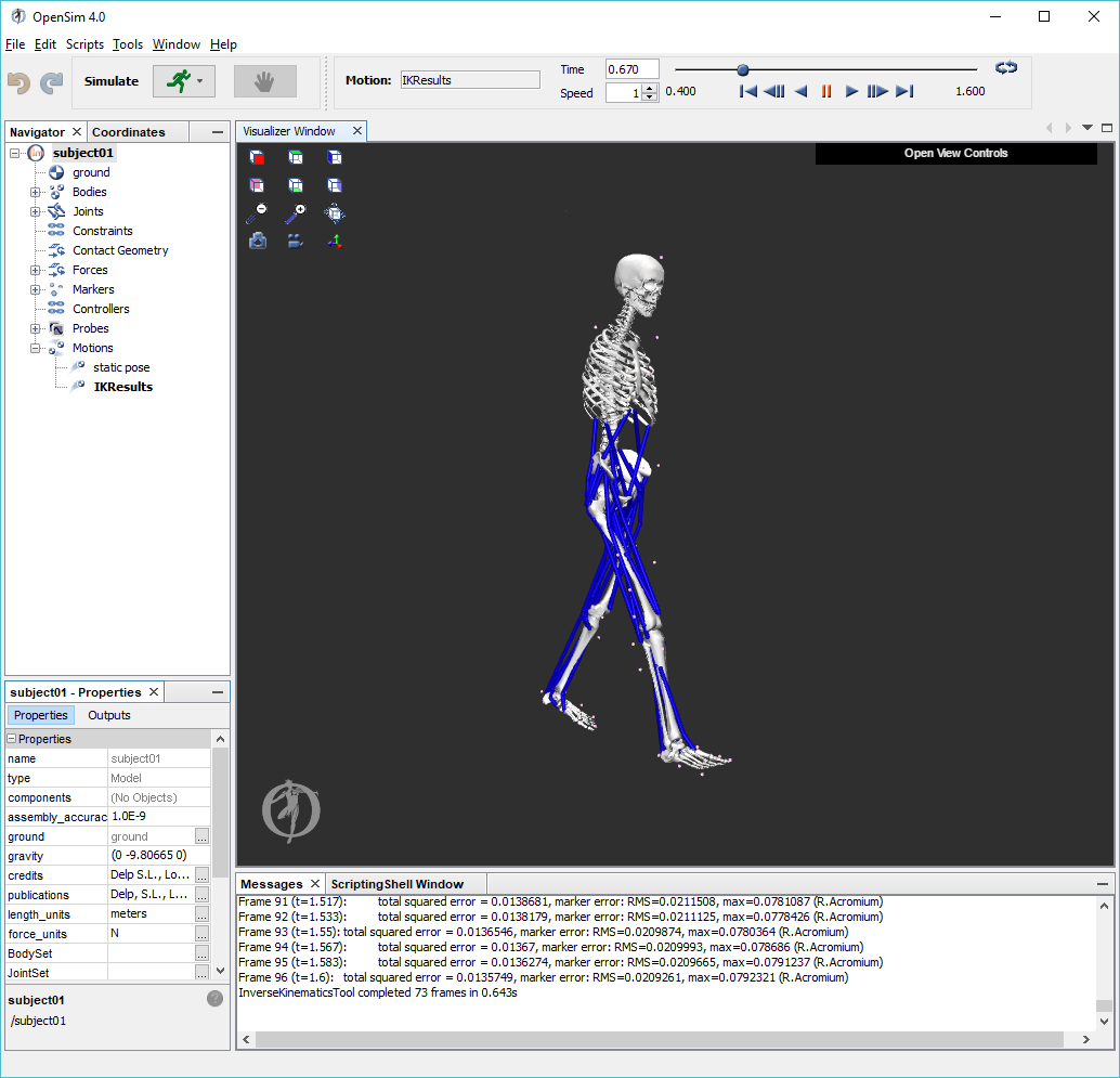
View which markers are selected for use in the inverse kinematics analysis, and their corresponding weights.
Enable the tracking for the marker R.Knee.Lat. Notice the row turns red and the Run button is now greyed out. You will be unable to run the inverse kinematics tool because there is no experimental data found for the R.Knee.Lat marker in the subject_walk1.trc file. Disable the R.Knee.Lat marker and notice the Run button is now clickable.

To perform inverse kinematics:

Click Run. The model will begin to move as the inverse kinematics problem is being solved for each frame of the experimental data.
Notice the progress bar in the lower right-hand corner of the program. Wait until the bar disappears before proceeding.
Note: Closing the inverse kinematics tool dialog during the analysis doesn't affect the Inverse Kinematics tool running.

To visualize the inverse kinematics solution, animate the model by using the motion slider and video controls. The model should walk through one full gait cycle.
Note: You can loop and control the speed of the animation.
The inverse kinematics solution is saved to subject01_walk1_ik.mot, as specified in the setup file.
Note: Be sure to use the exact file name given, as this file is used later.
To compare experimental marker data with inverse kinematics results, in the Navigator panel, go to Motions and right-click on IKResults (which are what the Inverse Kinematics Tool just generated). Then choose Associate Motion Data... from the drop-down menu. Choose subject01_walk1.trc and click Open. Model markers are shown in pink and experimental markers are shown in blue. Hit play in the Motion Toolbar. The virtual markers should correspond closely to the experimental marker locations as the animation proceeds.
Note: If using a Virtual Machine on a Mac, Command + Ctrl + Left Click on each motion.
Click the Window menu and select Messages. The Messages window records details of all steps you have performed. Take a minute to explore the Messages window. Then, scroll to the very bottom. The line above InverseKinematicsTool completed... provides the markers errors and model coordinate errors (e.g., joint angle errors) associated with the last frame of the motion.
Note: All marker errors have units in meters, and all coordinate errors have units in radians.
Once you have answered Questions 4-6, below, close the Inverse Kinematics Tool Dialog by clicking Close.

Questions

4. In the inverse kinematics Tool dialog window, click the Weights tab and scroll through the list of markers in the top half of the weights tab. Which markers have weighting values less than one? Why?
Hint: Think about joints that have not been modelled.

5. Based on information in the Messages window, what is the root-mean-squared (RMS) error of all the markers in the last frame of the motion? Include units. Does this seem reasonable? Explain.

6. What was the value of the maximum marker error in the last frame? Include units. Which marker had this maximum error, and why?
Hint: Think about the weighted least squares problem.

V. Inverse Dynamics

Dynamics is the study of motion and the forces and moments that produce that motion. To perform inverse dynamics, estimation of mass and inertia is required. The purpose of inverse dynamics is to estimate the forces and moments that cause a particular motion, and its results can be used to infer how muscles are utilized in that motion. To determine these forces and moments, equations of motion for the system are solved iteratively [3]. The equations of motion are derived using the kinematic description and mass properties of a musculoskeletal model. Then, using the joint angles from inverse kinematics and experimental ground reaction force data, the net reaction forces and net moments at each of the joints are calculated such that the dynamic equilibrium conditions and boundary conditions are satisfied [3].

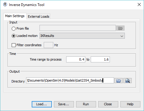
To setup an inverse dynamics analysis: Open the inverse dynamics tool dialog window by clicking the Tools menu and selecting Inverse Dynamics. Load an inverse dynamics tool setup file by clicking Load, selecting file *subject01_Setup_InverseDynamics.xml,* and clicking Open. Note: If the Motion From File textbox appears red, this means the textbox was filled with an inappropriate file name. Make sure the motion file was saved with the correct file name in the Inverse Kinematics section. Note the folder listed in the Directory textbox, located in the Output section of the dialog. The storage file containing the inverse dynamics results will be saved in this folder: Documents\Opensim\Models\Gait2354\ResultsInverseDynamics. A detailed explanation of the Inverse Dynamics Tool can be found on the Inverse Dynamics page of the documentation.
To perform inverse dynamics: Click Run. Notice the progress bar in the lower right-hand corner of the program. Wait until the bar disappears before proceeding. Note: Closing the inverse dynamics tool dialog during the analysis doesn't affect the Inverse Dynamics tool running. To visualize the inverse dynamics solution, animate the model by using the motion slider and video controls. The model should walk through one full gait cycle. Note: You can loop* and control the speed of the animation.* It is often useful to view the ground reaction forces with the inverse dynamics results. in the Navigator panel, go to Motions and right-click on IDResults (which are what the Inverse Dynamics Tool). Then choose Associate Motion Data... from the drop-down menu. Choose subject01_walk1_grf.mot and click Open. Green arrows are now shown that represent ground reaction force vectors collected from a force plate. Close the inverse dynamics tool dialog window.
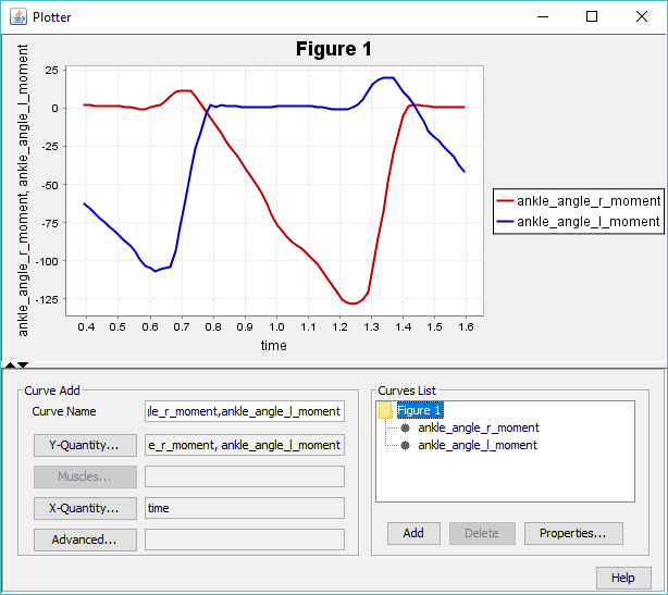
When completed, examine the results of the inverse dynamics solution by plotting the net moments at the left and right ankles: Click Tools and select Plot. In the Plotter window, click the Y-Quantity button and select Load File. In the file browser, go to the ResultsInverseDynamics folder, select the file *inverse_dynamics.sto, and click Open. In the menu, select ankle_angle_r_moment* and ankle_angle_l_moment by clicking the corresponding checkboxes, then click OK. Note: To quickly find these quantities, type ankle into the pattern text box. Click the X-Quantity button, select time, and click OK. Back in the Plotter window, click Add to add the moment curves to the plot. Print your plot by right clicking on the plot and selecting Print. Note: To export the plot as an image by right-clicking* the plot and selecting Export Image.* After printing the plot and answering questions 7-8, Close the Plotter and inverse dynamics dialog window
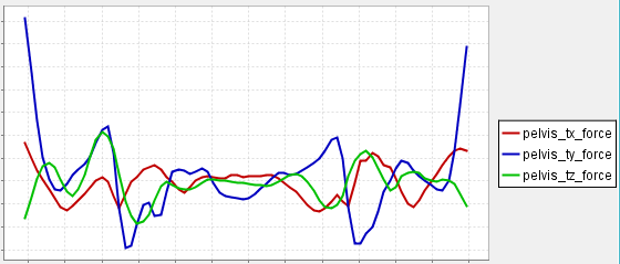
In solving the inverse dynamics problem, both kinematic data and force plate data were used, making this an over-determined problem. In other words, the problem has more equations than unknowns (i.e., degrees of freedom). Due to errors in the experimental motion data and inaccuracies in the musculoskeletal model, it turns out that Newton's second law is violated, or [3]. One method to handle this inconsistency is to compute and apply residual forces and moments to a particular body segment in the model, such that Newton's second law becomes: † An analogous equation relates the ground reaction moment, to the residual moment, . In this musculoskeletal model, the residuals are applied to the pelvis segment. To see the residuals from the inverse dynamics solution, in a new plot window, Plot pelvis_tx_force, pelvis_ty_force, and pelvis_tz_force versus time. Using this plot, answer question 9. While applying residual forces and moments makes the model's motion dynamically consistent with the external forces , this strategy is undesirable because the residuals can be large. More advanced strategies have been developed to deal with the problem of residuals and dynamic inconsistencies, such as least-squares optimization [3], the Residual Elimination Algorithm (REA) [5], and the Residual Reduction Algorithm (RRA) [6]. OpenSim implements a Residual Reduction Algorithm as part of its workflow for generating muscle-actuated simulations [6]. A detailed explanation of the Residual Reduction Algorithm (RRA) can be found on the Residual Reduction Algorithm page of the documentation. For additional information on these strategies, please also see [3], [5], [6], and [7].

Questions

7. On your plot of the ankle moments, identify when heel strike, stance phase, toe off, and swing phase occur for each curve (i.e., left leg and right leg).

8. Based on your plot and the angle convention for the ankle, give an explanation of what is happening at the ankle just before toe-off.
Hint: It may be useful to use the Coordinate sliders to understand the angle convention for the ankle.

9. What are the maximum magnitudes of the residual forces? Using the mass of the subject from Question 1, what fraction of body weight are the maximum residual forces?

Acknowledgements

The experimental gait data were collected by Jill Higginson and Chand John in the Neuromuscular Biomechanics Lab at the University of Delaware [8]. The data include marker trajectories and ground reaction forces for an adult male walking at a self-selected speed on an instrumented split-belt treadmill. Please note that the data distributed with OpenSim is from a different subject than the one described in the paper. Data collection protocols were the same for both subjects.

References

1. Delp, S.L., Loan, J.P., Hoy, M.G., Zajac, F.E., Topp E.L., Rosen, J.M. An interactive graphics-based model of the lower extremity to study orthopaedic surgical procedures. IEEE Transactions on Biomedical Engineering, vol. 37, pp. 757-767, 1990.

2. Anderson, F.C., Pandy, M.G. A dynamic optimization solution for vertical jumping in three dimensions. Computer Methods in Biomechanical and Biomedical Engineering, vol. 2, pp. 201-231, 1999.

3. Kuo, A.D. A least squares estimation approach to improving the precision of inverse dynamics computations, Journal of Biomechanical Engineering, vol. 120, pp. 148-159, 1998.

4. Winter, D.A. Biomechanics and Motor Control of Human Movement, Wiley and Sons, pp. 77-79, 1990.

5. Thelen, D.G., Anderson, F.C. Using computed muscle control to generate forward dynamic simulations of human walking from experimental data, Journal of Biomechanics, vol. 39, pp. 1107-1115, 2006.

6. John, C.T., Anderson, F.C., Guendelman, E., Arnold, A.S., Delp, S.L. An algorithm for generating muscle-actuated simulations of long-duration movements, Biomedical Computation at Stanford (BCATS) Symposium, Stanford University, 21 October 2006, Poster Presentation.

7. Delp, S.L., Anderson, F.C., Arnold, A.S., Loan, P., Habib, A., John, C.T., Guendelman, E., Thelen, D.G. OpenSim: Open-source software to create and analyze dynamic simulations of movement. IEEE Transactions on Biomedical Engineering, vol. 55, pp. 1940-1950, 2007.

8. Chand T. John, Frank C. Anderson, Jill S. Higginson & Scott L. Delp (2012): Stabilisation of walking by intrinsic muscle properties revealed in a three-dimensional muscle-driven simulation, Computer Methods in Biomechanics and Biomedical Engineering.